3  Temporal Logic

Temporal logic assigns a truth value to a variable at each point in time.

A Kripke structure is a state transition system mathematically defined as M = (S, I, R, L) where

• S is a set of states

• I \subseteq S is a set of initial states

• R \subseteq S \times S is a set of state transition relations: \foralls \in S, there is s^{'} such that s \rightarrow s^{'} defined as (s, s^{'}) \in R

• L is a labelling function that maps S to the power set of \Sigma, where \Sigma is the set of atomic propositions. L(s) is a set of all atomic propositions that are evaluated to true in the state s

The transition system is graphically represented as a directed graph, in which each node is a state, state transitions are depicted by directed arrows, and the labelling is marked on the node.

The definition of R indicates that each computation path is infinite. If a state that represents a deadlock situation exists, then we can draw an outgoing edge back to the state itself.

3.1 Time modelling

There are two models of time.

• Linear model: time is represented as a structure (T, <), where T is a set of time points and < is a precedence relation on T. If a pair (s, t) belongs to <, s is earlier than t. For a point s, the set {t \in T | s < t} is the future of s, the past is defined likewise.

• Branching model: a time point r may have two or more future time points that are not related to each other; the future of r is non deterministic.

3.2 Linear Temporal Logic (LTL)

3.2.1 Syntax

LTL extends propositional logic introducing a set of temporal operators.

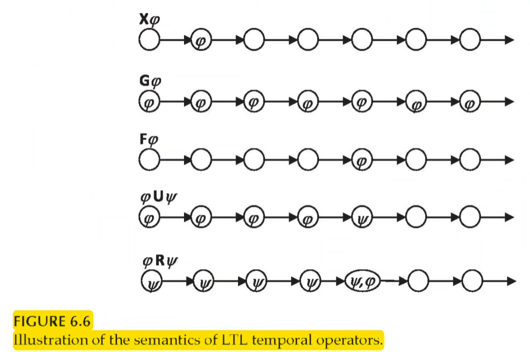
• \mathcal{X} means neXt state. \mathcal{X} p is true if p is true in the next state

• \mathcal{F} means some Future state. \mathcal{F} p is true if there is a reachable future where p is true

• \mathcal{G} means all future states (globally). \mathcal{G} p is true if p is true in all future states (also in the current)

• \mathcal{U} means Until. p \mathcal{U} q is true if p is true until q is true in a future state

• \mathcal{R} means Release. p \mathcal{R} q is true if q is true until the first state in which p is true

Unary operators bind equally strongly.

\mathcal{U} and \mathcal{R} bind more strongly than \land and \lor.

\rightarrow has the least binding priority.

An LTL formula is well-formed iff it obeys the following inductive construction rules:

• True and false are LTL formulas

• Any atomic propositional formula is an LTL formula

• If \varphi and \psi are LTL formulas, then so are \neg \varphi, \varphi \land \psi, \varphi \lor \psi and \varphi \rightarrow \psi

• If \varphi and \psi are LTL formulas, then so are \mathcal{X} \varphi, \mathcal{F} \varphi, \mathcal{G} \varphi, \varphi \mathcal{U} \psi, and \varphi \mathcal{R} \psi

3.2.2 Semantics

Consider a computation path \pi = s_1 \rightarrow s_2 \rightarrow \ldots which start from s_1, and denote by \pi_i the path starting with s_i \pi = s_i \rightarrow s_{i + 1} \rightarrow \ldots we define the satisfaction relation denoted by \vDash.

For any single atomic proposition p \in \Sigma \pi \vDash p \iff p \in L(s_1)

Any composition of \varphi and \psi with propositional logic operators is evaluated in the first state s_1 of the path: 1. \pi \vDash \neg \varphi \iff \pi \not \vDash \varphi

2. \pi \vDash \varphi \land \psi \iff \pi \vDash \varphi and \pi \vDash \psi

3. \pi \models \varphi \lor \psi \iff \pi \models \varphi or \pi \models \psi

4. \pi \models \varphi \rightarrow \psi \iff \pi \models \psi as long as \pi \models \varphi

All LTL formulas that are composed with temporal operators should be evaluated across states.

5. \pi \models X\varphi \iff \pi_2 \models \varphi

   That is, iff \varphi is evaluated to true in the next state s_2, then we have \pi \models X\varphi.

6. \pi \models G\varphi \iff \pi_i \models \varphi for all i \geq 1

   That is, iff \varphi is evaluated to true in every state along the path \pi, then we have \pi \models G\varphi.

7. \pi \models F\varphi \iff \pi_i \models \varphi for some i \geq 1

   That is, iff \varphi is evaluated to true in some state along the path \pi, then we have \pi \models F\varphi.

8. \pi \models \varphi U \psi \iff \pi_i \models \psi for some i \geq 1 and \pi_j \models \varphi for all j = 1, 2, \ldots, i-1

   That is, iff \varphi is evaluated to true in every state along the path \pi until a state in which \psi is evaluated to true, then we have \pi \models \varphi U \psi. By the way, we can view F\varphi as an abbreviation of \top U \varphi.

9. \pi \models \varphi R \psi \iff \pi_i \models \varphi for some i \geq 1 and \pi_j \models \psi for all j = 1, 2, \ldots, i

   That is, iff \psi is evaluated to true under every state along the path \pi until a state under which both \varphi and \psi are evaluated to true, then we have \pi \models \varphi R \psi.

When we verify a system against an LTL formula from a state we check if the formula is satisfied by all paths from the state, so if \pi \vDash \varphi holds for every computation path \pi starting at the state s.

Two LTL formulas \varphi and \psi are said to be semantically equivalent, denoted by \varphi \equiv \psi, if for all models M and all states s in M M, s \models \varphi \iff M, s \models \psi Two formulas are equivalent if they are evaluated to the same truth value from any state of any computation path of any Kripke structure.

Listed below are a few equivalencies:

X(\varphi \land \psi) \equiv X\varphi \land X\psi

X(\varphi \lor \psi) \equiv X\varphi \lor X\psi

X(\varphi \text{ U } \psi) \equiv X\varphi \text{ U } X\psi

F(\varphi \lor \psi) \equiv F\varphi \lor F\psi

G(\varphi \land \psi) \equiv G\varphi \land G\psi

X\neg\varphi \equiv \neg X\varphi

F F\varphi \equiv F\varphi

G G\varphi \equiv G\varphi

\neg F\varphi \equiv G\neg\varphi

\neg(\varphi R \psi) \equiv \neg\varphi U \neg\psi

3.3 Computation Tree Logic (CTL)

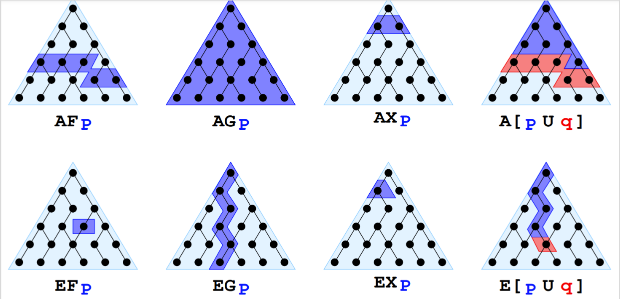
Branching-time structure introduces two temporal operators: \mathcal{A} (“for all paths”) and \mathcal{E} (“there exists a path”).

The inductive construction rules are the same, adding simply the two new operators.

The semantic is intuitively defined as follows: